Matlab code from Vannson et al., 2017 (paper here)
This code has been simplified for displaying purposes.
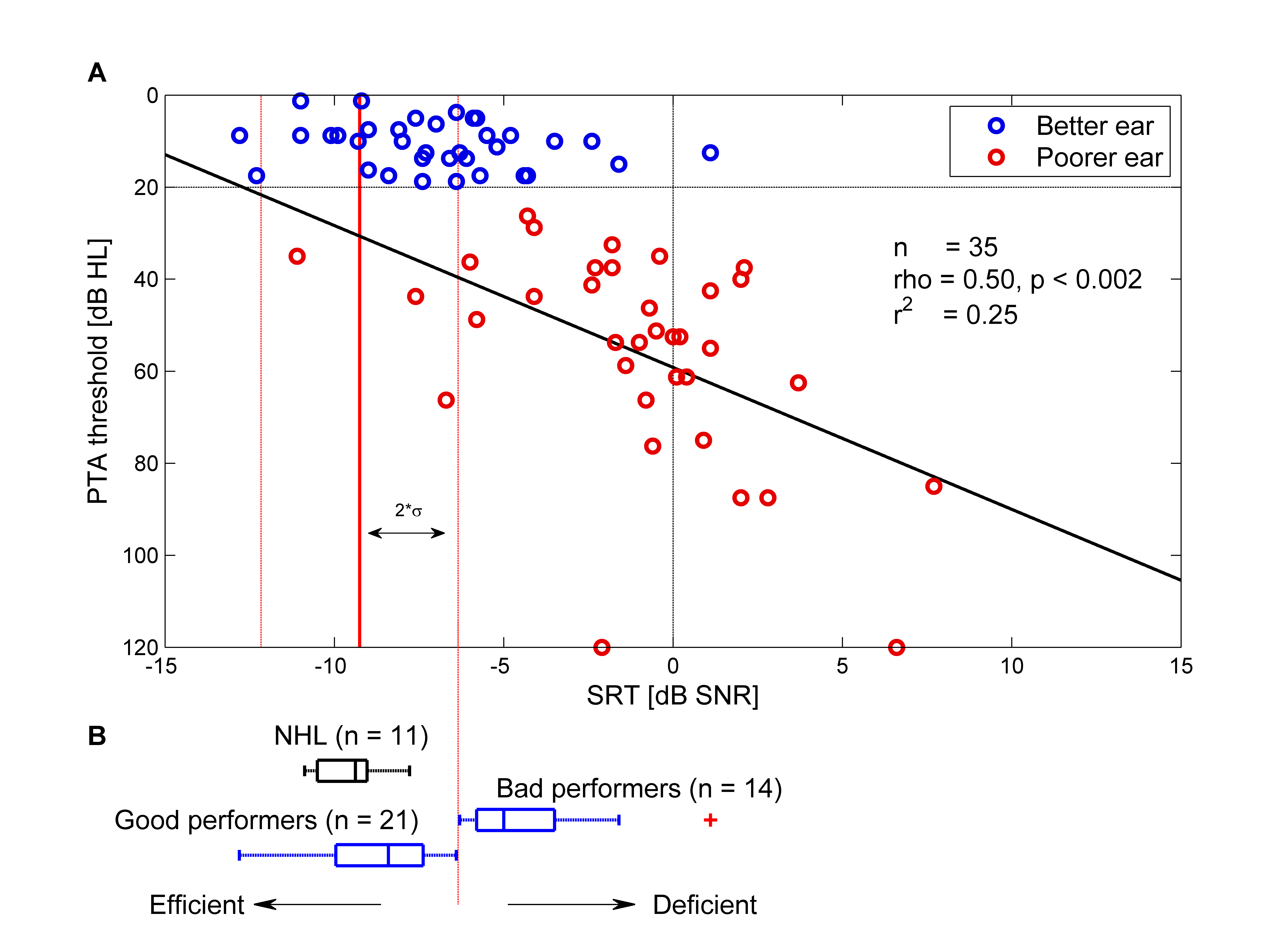
The primary objective of this study was to correlate speech-in-noise abilities with pure-tone audiometry in individuals with unilateral hearing loss, with the goal of developing a predictive model.
    % Binaural graph
    % NV, Toulouse , July 2014


    clear all
    close all
    clc

    % Cmd

    binaural = 1;   % 1 = Plot binaural graph
    matrix   = 1;   % 1 = Plot matrix graph
    keep     = 1;   % 1 = Save figure
    tostudy  = 2;  % group to compute

    % Param

    groups   = {'Binauralite' ,...
                'Binauralite-perdue' ,...
                'Binauralite-rehabilite', ...
                'Binauralite-rehabilite-NA',...
                'perdue-NA',...
                'TEMOINS'};


    source          = 'F:\NV_PhD\Data_sujets\Results';
    boris           = 'F:\NV_PhD\Data_Boris';
    mfile           = 'F:\NV_PhD\Tools\Matlab';
    img             = 'F:\NV_PhD\PhD_img';


    police          = 12;
    font            = 'bold';
    graph_ext       = '-dpng';
    reso            = '-r900';
    col             = [ 0.9 0 0 ; 0 0.7 0 ; 0 0 0.9 ;1 165/255 0;0.5 0.5 0.5; .8 .8 .8];

    % NV Norms (new both : n = 27)
    normes     = [-5.3154 -13.45 -13.45];
    std_normes = [0.6697  3.71 3.71];
    cutoff     = std_normes;


    % -------------------------------------------------------------------------

    % add mfile folder (matlab file)
    addpath(genpath(mfile))

    % Load data

    cd(source)
    folder  = [ pwd  filesep 'Groupe_' char(cellstr(groups(tostudy)))];
    name    = char(cellstr(groupes(tostudy)));
    sprintf('Group data loaded is :  %s', name)
    cd(folder)

    % Choose to load only audio and matrix data

    data       = load(['data_'  char(cellstr(groupes(tostudy))) '.mat']);
    audio      = data.data.audiometrie;  audiometry
    matrix     = data.data.matrix; Speech-in-noise data(Matrix)

    % Sort ears
    % check ears and rearrange them to put the better ear within the first column

    NHL_OD = audio(:,1);
    NHL_OG = audio(:,2);

    oreilles = [NHL_OD NHL_OG];
    for k = 1 : length(oreilles)

            if oreilles(k,1) >= 25
                oreilles(k,[1,2]) = oreilles(k,[2,1]);
            end

            if oreilles(k,1) > oreilles (k,2)
                oreilles(k,[1,2]) = oreilles(k,[2,1]);
            end
    end


    % Check for real uhl patients based upon oreilles (:,1)= < 20 dB

    deafness = [num2cell(oreilles) num2cell(matrix) num2cell(audio)];
    uhl = {[]};
    bhl = uhl;
    for i = 1: size(deafness,1)
        if  cell2mat(deafness(i,1)) <= 20
            uhl{i,1} = deafness(i,:);
        else
            bhl{i,1} = deafness(i,:);
        end
    end
    emptyCells = cellfun(@isempty,uhl);
    uhl(emptyCells) = [];
    emptyCells = cellfun(@isempty,BHL);
    bhl(emptyCells) = [];

    % Save uhl and bhl groups
    save uhl uhl
    save bhl bhl


    % Binaural graph
    % -------------------------------------------------------------------------

    if binaural == 1

        % Matrix limits
        normes = normes(1,2);
        cutoff = cutoff(1,2);


        % Matrix data : % dio - dicho - inv conditions

        x = [oreilles(:,1) matrix(:,3)];
        y = [oreilles(:,2) matrix(:,2)];

        figure
        set(gcf,'name',[titlegraphe,' ',name,' ',date],'numbertitle','off')
        set(gcf,'Toolbar','none','Menu','none');
        hold on
        box on

         % gca
        set(gca,'ydir','reverse')
        axis([-15 15 0 120])
        set(gca,'position',[0.13,0.32,.8,0.58]);

         % line
        line ([ normes  normes],[ 0 120],'linestyle','-','color','r')
        line ([ normes+cutoff normes+cutoff],[ 0 120]'linestyle','--','color','r')
        line ([ normes-cutoff  normes-cutoff ],[ 0 120],'linestyle','--','color','r')
        line ([ 0 0 ],[ 0 120],'linestyle','--','color','k')
        line ([min(xlim) max(xlim)],[20  20],'linestyle','--','color','k')


        % plot pts
        hbo = plot(uhl(:,5),uhl(:,1),'ob','markersize',6,'LineWidth',2,'markeredgecolor',col(3,:));
        hmo = plot(uhl(:,4),uhl(:,2),'or','markersize',6,'LineWidth',2,'markeredgecolor',col(1,:));

        % Multiple correlation analysis
        [rmat,~,pmat]   = spear(matrix(:,2),matrix(:,3));
        [rbad,~,pbad]   = spear(uhl(:,2),uhl(:,4))
        [rgood,~,pgood] = spear(uhl(:,1),uhl(:,5))

        % Fitting on only the bad ears
        [cbad,gbad] = fit(uhl(:,4),uhl(:,2),'poly1','robust','Off');
        pp = plot(cbad,'k');
        set(pp,'linewidth',1.5);
        legend off

        % info
        text(6.5,40,sprintf('rho = %2.2f, p < %2.3f',rbad,pbad),'fontsize',police)
        text(6.5,47,sprintf('r^2    = %2.2f',rbad*rbad),'fontsize',police)
        text(6.5,33,sprintf('n     = %2.0f',size(uhl,1)),'fontsize',police)

        % labels & legend
        ylabel('PTA threshold [dB HL]','fontsize',police)
        xlabel('SRT [dB SNR]','fontsize',police)
        legend off
        legend([hbo,hmo],{'Better ear';'Poorer ear'},'fontsize',police)

        text('string','2*\sigma','HorizontalAlignment','center','position',[-7.8 90],'fontsize',police-4)
        text('string','A','HorizontalAlignment','center','position',[-17 -5],'fontsize',police,'fontweight','bold')

        annotation('doublearrow',  [.29 .35], [.44 .44],...
            'Head1Length',police-6,'Head1Width',police-6,...
            'Head2Length',police-6,'Head2Width',police-6);


        % boxplot beneath
        hl = axes('position',[0.13,0.05,0.8,0.3]);
        set(gca,'ydir','reverse')
        axis([-15 15 0 120])
        axis off
        line ([ normes+cutoff normes+cutoff],[ 0 120],'linestyle','--','color','r')


        %  add boxplot on the bottom
        htop = axes('position',[0.13,0.08,0.8,0.2]);
        p = boxplot(htop,in(:,5),'color','b','position',-10,'width',3,'orientation','horizontal');
        set(p,'linewidth',1.5)
        hold on
        p = boxplot(htop,out(:,5),'position',-5,'color','b','width',3,'orientation','horizontal');
        set(p,'linewidth',1.5)
        % add nhl to the boxplot graph
        ndata = mean(nhl(:,2:3),2);
        p = boxplot(htop,ndata,'position',2,'color','k','width',3,'orientation','horizontal');
        set(p,'linewidth',1.5);
        set(gca,'XTickLabel',{' '},'YTickLabel',{' '})
        axis([-14.66 15  -14 14])
        axis off


        text('string','NHL (n = 11)','HorizontalAlignment','center','position',[-9.5 7],'fontsize',police)
        text('string','Good performers (n = 21)','HorizontalAlignment','center','position',[-12 -5],'fontsize',police)
        text('string','Bad performers (n = 14)','HorizontalAlignment','center','position',[-1 -.5],'fontsize',police)
        text('string','B','HorizontalAlignment','center','position',[-17 7],'fontsize',police,'fontweight','bold')

        % Create textboxs & arrows

        annotation(gcf,'textbox',...
        [0.15 0.05 0.01 0.020],...
        'String',{'Efficient'},...
        'HorizontalAlignment','center',...
        'fontsize',police,...
        'LineStyle','none');

        annotation(gcf,'textbox',...
        [0.55 0.05 0.01 0.020],...
        'String',{'Deficient'},...
        'HorizontalAlignment','center',...
        'fontsize',police,...
        'LineStyle','none');

        annotation(gcf,'arrow',[0.4 0.5],...
        [0.05 0.05],'HeadWidth',6,'LineWidth',0.6);
        annotation(gcf,'arrow',[0.3 0.2],...
        [0.05 0.05],'HeadWidth',6,'LineWidth',0.6);


        % savefig
        if keep == 1
            cd(pwd)
            print(graph_ext,reso,'PTAvsSRT')
        end
    % Matrix good vs bad performers
    % -------------------------------------------------------------------------


    Based upon the previous binaural graph, sort patients into good and bad performers
    for further analysis and plot their Matrix results! The sorting will depend on the
    better ear SRT (matrix) score.


    Filter out uhl data to find uhl in and uhl out patients
    out = uhl*0;
    in  = uhl;  % to discard out data
    for j = 1 : size(uhl)
        if uhl(j,1) <= 20 & uhl(j,5)> (normes+cutoff)
            out(j,:) =  uhl(j,:);
        end
    end

    idxo                = out(:,1) == 0;
    out(idxo,:)         = [];
    in(out(:,end),:)    = [];

    % Save in and out groups
    save in in
    save out out


    if matrix == 1

        % From Boris : load nhl data
        addpath(genpath(boris))
        nhl  = load('Boris_NHL_matrix.txt');
        nhl  = nhl(:,1:3);  % dio - dicho - inv

        % gather dicho _inv
        dicho = [nhl(:,2) nhl(:,3)];
        dicho = mean(dicho,2);

        % plot param
        leg         = {'Dichotic','Diotic','Reversed dichotic '};
        xlabeltxt   = 'Subjects';
        ylabeltxt   = 'SRT [dB SNR] ';
        deaf_ear    = 'impaired ear';
        titlegraph  = 'Matrix test';
        mk          = 8; % marker size

        % figure
        figure
        set(gcf,'Toolbar','none','Menu','none');
        set(gca,'LooseInset',get(gca,'TightInset'))
        hold on
        box on

        % plot nhl data (dio - dicho - inv)
        hnhl = plot(1,dicho,'ok','markersize',mk);
        plot(5,nhl(:,1),'ok','markersize',mk)
        plot(9,dicho,'ok','markersize',mk)

        % boxplots
        % plot all point first
        hin = plot(2,in(:,4),'ob','markersize',mk);
        plot(6,in(:,3),'ob','markersize',mk)
        plot(10,in(:,5),'ob','markersize',mk)

        hout = plot(3,out(:,4),'or','markersize',mk);
        plot(7,out(:,3),'or','markersize',mk)
        plot(11,out(:,5),'or','markersize',mk)

        % dicho
        boxplot(dicho,'position',1,'color','k','width',.5) % dicho
        set(gca,'XTickLabel',{' '})
        boxplot(in(:,4),'position',2,'color','k','width',.5)
        set(gca,'XTickLabel',{' '})
        h = boxplot(out(:,4),'position',3,'color','k','width',.5);
        set(h(7,:),'Visible','off') ;
        set(gca,'XTickLabel',{' '})

        % dio
        boxplot(nhl(:,1),'position',5,'color','k','width',.5) % dio
        set(gca,'XTickLabel',{' '})
        h = boxplot(in(:,3),'position',6,'color','k','width',.5);
        set(h(7,:),'Visible','off') ;
        set(gca,'XTickLabel',{' '})
        h = boxplot(out(:,3),'position',7,'color','k','width',.5);
        set(h(7,:),'Visible','off') ;
        set(gca,'XTickLabel',{' '})

        % Inv
        nl = boxplot(dicho,'position',9,'color','k','width',.5); % inv
        set(gca,'XTickLabel',{' '})
        il = boxplot(in(:,5),'position',10,'color','k','width',.5);
        set(gca,'XTickLabel',{' '})
        ol = boxplot(out(:,5),'position',11,'color','k','width',.5);
        set(ol(7,:),'Visible','off') ;
        set(gca,'XTickLabel',{' '})

        ylabel('SRT [dB SNR]','fontsize',police)
        axis([0 12 -20 20])

        % bootstrap stats
        st_inv_out     = bootci(10000,@mean, out(:,5));
        st_inv_in      = bootci(10000,@mean, in(:,5));
        st_inv_nhl     = bootci(10000,@mean, nhl(:,3));

        st_dicho_out   = bootci(10000,@mean, out(:,4));
        st_dicho_in    = bootci(10000,@mean, in(:,4));
        st_dicho_nhl   = bootci(10000,@mean, nhl(:,2));

        st_dio_nhl     = bootci(10000,@mean, nhl(:,1));
        st_dio_out     = bootci(10000,@mean, out(:,3));
        st_dio_in      = bootci(10000,@mean, in(:,3));


        % Display stats results
        % text

        % dicho
        text('string','*','HorizontalAlignment','center','position',[1.5 6],'fontsize',police+2)
        text('string','*','HorizontalAlignment','center','position',[2.5 11],'fontsize',police+2)
        text('string','*','HorizontalAlignment','center','position',[2 14],'fontsize',police+2)

        % dio
        text('string','*','HorizontalAlignment','center','position',[5.5 6],'fontsize',police+2)
        text('string','*','HorizontalAlignment','center','position',[6.5 10],'fontsize',police+2)
        text('string','*','HorizontalAlignment','center','position',[6 14],'fontsize',police+2)

        % inv
        text('string','N.S','HorizontalAlignment','center','position',[9.5 -3],'fontsize',police-1) % inv
        text('string','*','HorizontalAlignment','center','position',[10.5 4],'fontsize',police+2) % inv
        text('string','*','HorizontalAlignment','center','position',[10 11],'fontsize',police+2) % inv


        % line
        line([1 2],[5 5],'linestyle','-','color','k','linewidth',1.1)
        line([2 3],[10 10],'linestyle','-','color','k','linewidth',1.1)
        line([1 3 ],[13 13],'linestyle','-','color','k','linewidth',1.1)

        line([5 6],[5 5],'linestyle','-','color','k','linewidth',1.1)
        line([6 7],[9 9],'linestyle','-','color','k','linewidth',1.1)
        line([5 7 ],[13 13],'linestyle','-','color','k','linewidth',1.1)

        line([9 10],[-4.5 -4.5],'linestyle','-','color','k','linewidth',1.1)
        line([10 11],[3 3],'linestyle','-','color','k','linewidth',1.1)
        line([9 11],[10 10],'linestyle','-','color','k','linewidth',1.1)


        set(gca,'position', [0.1675,0.1285,0.76,0.40])

        % legend
        legend([hnhl(3,1);hin(4,1);hout(5,1)],...
        {'NHL (n = 11)','Good performers (n = 21)','Bad performers (n = 14)'},'fontsize',police-1)
        legend boxoff
        set(legend,'position',[0.43 0.41 0.2 0.3],'orientation','horizontal')

        % add details to the figure
        set(gca,'Xtick',[2,6,10])
        text('string','S_P_EN_B_E','HorizontalAlignment','center','position',[2 -24.5],'fontsize',police-1)% dicho
        text('string','S_F_R_O_N_TN_F_R_O_N_T','HorizontalAlignment','center','position',[6 -24.5],'fontsize',police-1)%dio
        text('string','N_P_ES_B_E','HorizontalAlignment','center','position',[10 -24.5],'fontsize',police-1) % inv

        % add conditions
        text('string',leg(1)','HorizontalAlignment','center','position',[2 -22],'fontsize',police-1)% dicho
        text('string',leg(2),'HorizontalAlignment','center','position',[6 -22],'fontsize',police-1)%dio
        text('string',leg(3),'HorizontalAlignment','center','position',[10 -22],'fontsize',police-1) % inv


        % imgs
        addpath(genpath(img))
        folder  = dir(fullfile(img,'ENG_*.png'));
        dicho   = imread(folder(1).name,'BackgroundColor',[1 1 1]);
        dio     = imread(folder(2).name,'BackgroundColor',[1 1 1]);
        inv     = imread(folder(3).name,'BackgroundColor',[1 1 1]);

        hold on
        haxinv   = axes('Position', [.165, .62, .24, .24]);
        imshow(dicho)
        haxdicho = axes('Position', [.425, .62, .24, .24]);
        imshow(dio)

        % legend for schemes
        hold on
        scatter(100,280,'ok','filled')
        ht = text(150,280,deaf_ear,'fontweight','normal','fontsize', police-1,'color','k');
        haxdio   = axes('Position', [.685, .62, .24, .24]);
        imshow(inv)


        % add textbox & arrows

        % Create textbox
        annotation(gcf,'textbox',...
        [0.045 0.17 0.01 0.020],...
        'String',{'Efficient'},...
        'HorizontalAlignment','center',...
        'fontsize',police,...
        'LineStyle','none');

        % Create textbox
        annotation(gcf,'textbox',...
        [0.045 0.47 0.01 0.020],...
        'String',{'Deficient'},...
        'HorizontalAlignment','center',...
        'fontsize',police,...
        'LineStyle','none');

        % Create arrow
        annotation(gcf,'arrow',[0.05 0.05],...
        [0.30 0.230],'HeadWidth',8,'LineWidth',0.8);

        % Create arrow
        annotation(gcf,'arrow',[0.05 0.05],...
        [0.35 0.42],'HeadWidth',8,'LineWidth',0.8);

        %savefig
        if keep == 1
            cd(art_folder)
            print(graph_ext,reso,['Matrix_NHL_' date])
        end
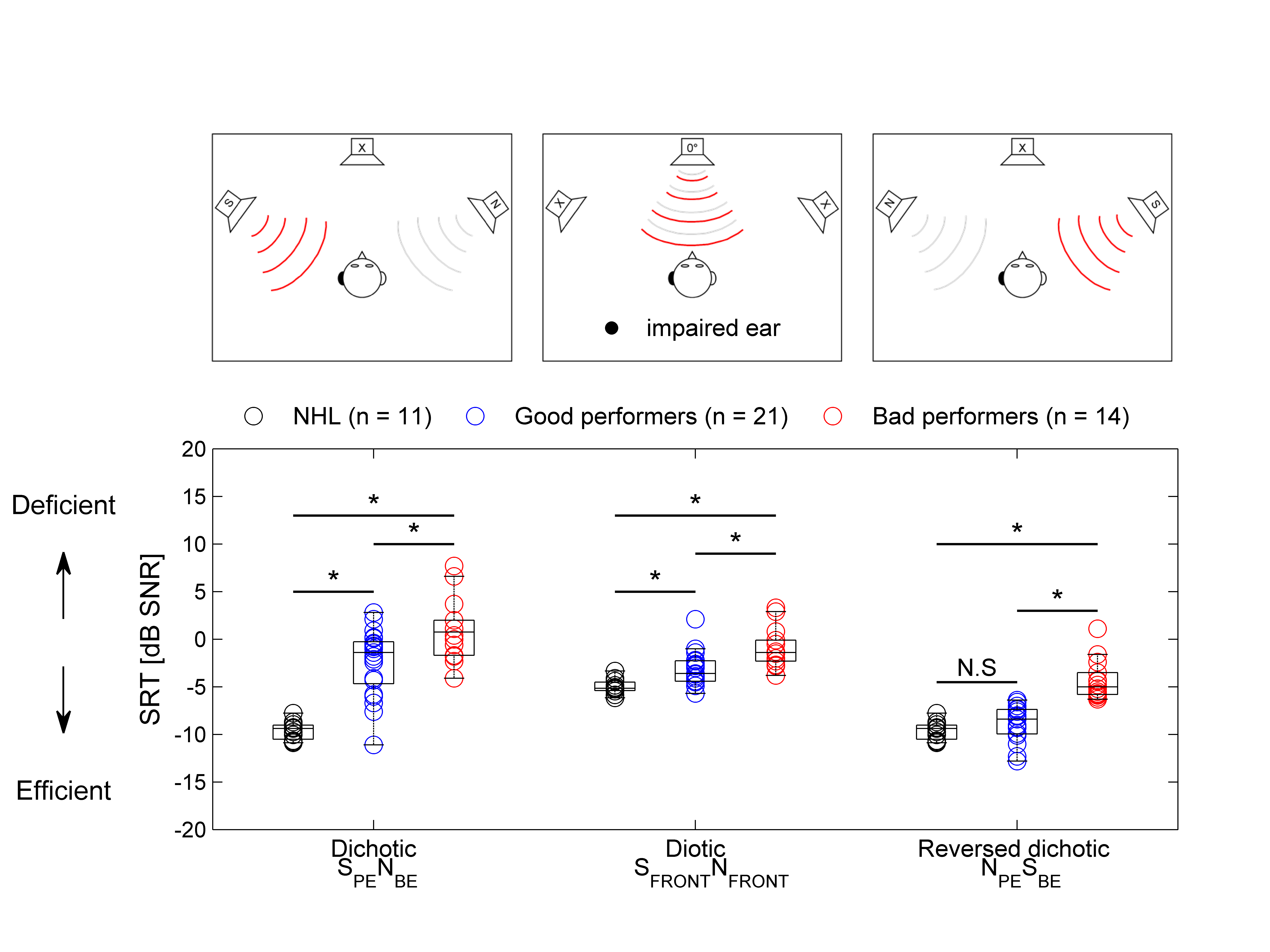
The code continues to deepen our understanding of how good and bad performers differ.